Inference with nonprobability samples

Author

Camilla Salvatore

Introduction

This material is part of the Utrecht Summer School S16 - Survey Research: Statistical Analysis and Estimation.

In this practical session we learn how to do inference with nonprobability samples; in the first part we discuss frequentist approaches (Inverse probability weighting, mass imputation and doubly robust methods) and in the second part the Bayesian MRP.

Frequentist approaches

In these exercises we use the nonprobsvy package developed by Maciej Beręsewicz and Łukasz Chrostowski. You can find additional information about the package here:

Basic use cases of the nonprobsvy package;
Modern inference methods for non-probability samples with R;
GitHub repository;
A video of a workshop on nonprobsvy.

The data

In this exercise, we will analyze data from the 2003 U.S. Michigan Behavioral Risk Factor Surveillance Survey, available in the PracTools package. The dataset, named mibrfss, includes various demographic and health-related variables. We use this dataset as the basis in order to simulate a population of size 100000 and different sampling scenarios. In particular, the data we provide you with are:

Population Totals: pop_tot.rda – Contains population totals.
Probability Sample (PS): p_sample.rda – A high-quality sample of size 10,000, assumed to be a simple random sample.
Non-Probability Sample (NPS): np_sample.rda – A sample of size 1,000 with self-selection and coverage issues.

We consider a subset of the variables available in the mibrfss dataset, namely:

SMOKE100 : Smoked 100 or more cigarettes in lifetime (1 = Yes; 2 = No)
AGECAT : Age group (1 = 18-24 years; 2 = 25-34 years; 3 = 35-44 years; 4 = 45-54 years; 5 = 55-64 years; 6 = 65+)
INETHOME : Has access to the Internet at home (1 = Yes; 2 = No)
EDCAT : Education level (1 = Did not graduate high school; 2 = Graduated high school; 3 = Attended college or technical school; 4 = Graduated from college or technical school)

For this exercise, we assume that the non-probability sample (NPS) was collected through social media advertisements. This approach introduces potential biases because only individuals with internet access and who are active on the specific social media platform could participate. Consequently, the NPS may suffer from both self-selection bias and coverage bias (since the sample is restricted to those with internet access and a presence on social media).

In contrast, we assume that the probability sample (PS) was obtained through a simple random sampling method. This sample is considered a high-quality reference sample, and for simplicity, we do not need to account for any design or calibration weights.

Objectives

Estimate the proportion of U.S. individuals aged 18+ who smoked 100 or more cigarettes in their lifetime
Compare different estimation techniques against the true population value of 52.85%

Preliminary analyses

Before starting, load the necessary R packages:

library(tidyverse)
library(ggplot2)
library(survey)
library(nonprobsvy)
library(PracTools)

Import and prepare the data: Load the datasets and inspect the data. Pay attention to the data format.

load("p_sample.rda")
load("np_sample.rda")
load("pop_tot.rda")

Task: Familiarize yourself with the datasets.

Note

The PS survey does not contain the target variable of interest, i.e., SMOKE100
You might encounter some issues when the variables are categorical. I suggest to save binary variables as numeric and variables with more than one level as character.
Pay attention to the pop_tot structure. It contains the population totals and it is formatted in order to match the nonprobsvy and survey package naming terminology. The (Intercept) simply contains the size of the population.

pop_tot

(Intercept)     AGECAT2     AGECAT3     AGECAT4     AGECAT5     AGECAT6 
     100000       13408       19554       22526       16875       21879 
   RACECAT2    RACECAT3      EDCAT2      EDCAT3      EDCAT4   INETHOME1 
       8255        5113       30925       28464       31668       65370

Compare the distribution of the covariates in the probability and nonprobability samples:

You can use prop.table.

Click here to show the solution

# Age
prop.table(table(p_sample$AGECAT))


     1      2      3      4      5      6 
0.0564 0.1351 0.1992 0.2211 0.1718 0.2164

prop.table(table(np_sample$AGECAT))


    1     2     3     4     5     6 
0.126 0.143 0.219 0.241 0.152 0.119

# Race
prop.table(table(p_sample$RACECAT))


     1      2      3 
0.8699 0.0792 0.0509

prop.table(table(np_sample$RACECAT))


    1     2     3 
0.878 0.061 0.061

# Education
prop.table(table(p_sample$EDCAT))


     1      2      3      4 
0.0875 0.3109 0.2801 0.3215

prop.table(table(np_sample$EDCAT))


    1     2     3     4 
0.111 0.256 0.267 0.366

# Internet at home
prop.table(table(p_sample$INETHOME))


   0    1 
0.35 0.65

prop.table(table(np_sample$INETHOME))


   0    1 
0.04 0.96

Individuals in the nonprobability samples are more young, with more graduated from collage or technical school higher education and mainly with internet at home.

Define the sampling desing: Specify the sampling designs for both the PS and NPS samples using the svydesign function.

Click here to show the solution

ps_design <- svydesign(ids = ~ 1,data = p_sample)

Warning in svydesign.default(ids = ~1, data = p_sample): No weights or
probabilities supplied, assuming equal probability

nps_design <- svydesign(ids = ~ 1,data = np_sample)

Warning in svydesign.default(ids = ~1, data = np_sample): No weights or
probabilities supplied, assuming equal probability

Estimate Proportion from Non-Probability Sample

Use the svymean and/or svyciprop functions to calculate the proportion and its confidence interval. Save it in a compare tibble where you will add the estimates obtained with different methods.

Click here to show the solution

svymean(~ SMOKE100, nps_design)

          mean     SE
SMOKE100 0.489 0.0158

np_est=svyciprop(~ SMOKE100, nps_design)
np_est

                2.5% 97.5%
SMOKE100 0.489 0.458  0.52

ci=confint(svyciprop(~ SMOKE100, nps_design))
compare = tibble(estimate=np_est[1], 
                lower_bound=ci[1],
                upper_bound=ci[2], 
                method="nps")

The estimate of the proportion of individuals who smoked 100 or more cigarettes in their lifetime from the non-probability sample (NPS) is 48.9%, with a 95% confidence interval ranging from 45.8% to 52.0%. Note that the confidence interval does not include the true population proportion.

To improve our estimate, we will apply and compare various estimation techniques.

Inverse-probability weighting

When a probability sample is available

First, we assume that we have access to high quality data from a reference probability sample. Implement IPW using the nonprob function with the following specifications:

Set up a selection model that includes the variables AGECAT, RACECAT, EDCAT, and INETHOME
Use as target variable SMOKE100
Use the probability sample design you created before as input for svydesign
Use logistic regression in method_selection
Save the estimate and the confidence interval

Click here to show the solution

ipw_logit_ps <-
  nonprob(
    selection = ~ as.factor(AGECAT) + as.factor(RACECAT) + as.factor(EDCAT) + as.factor(INETHOME),
    target = ~ SMOKE100,
    data = np_sample,
    svydesign  = ps_design,
    method_selection = "logit"
  )

#display
cbind(ipw_logit_ps$output, ipw_logit_ps$confidence_interval)

              mean         SE lower_bound upper_bound
SMOKE100 0.5302948 0.03644835   0.4588573   0.6017322

#save
compare <- compare %>% 
  bind_rows(tibble(estimate=ipw_logit_ps$output$mean, 
                lower_bound=ipw_logit_ps$confidence_interval$lower_bound,
                upper_bound=ipw_logit_ps$confidence_interval$upper_bound, 
                method="ipw_ps"))

The estimate is 53.02% (CI: 45.88% - 60.17%). This estimate is much closer to the true population proportion of 52.85%, and the confidence interval now includes the true value.

When only population information is available

Now we assume that only population totals are available.

Implement IPW using the nonprob function with the previous specifications but instead of svydesign , specify the pop_totals.

Click here to show the solution

ipw_logit_poptotals <-
  nonprob(
  selection =  ~ AGECAT + RACECAT + EDCAT + INETHOME,
  target = ~ SMOKE100,
  data = np_sample,
  pop_totals = pop_tot,
  method_selection = "logit"
  )

#display
cbind(ipw_logit_poptotals$output, ipw_logit_poptotals$confidence_interval)

              mean         SE lower_bound upper_bound
SMOKE100 0.5449075 0.07954355    0.389005     0.70081

#save
compare <- compare %>% 
  bind_rows(tibble(
    estimate = ipw_logit_poptotals$output$mean,
    lower_bound = ipw_logit_poptotals$confidence_interval$lower_bound,
    upper_bound = ipw_logit_poptotals$confidence_interval$upper_bound,
    method = "ipw_pop_tot"
  ))

Now, the estimate is 54.49% but the confidence interval is quite large (CI: 38.9% - 70%). This wide interval suggests considerable uncertainty in the estimate.

Mass Imputation

When a probability sample is available

First, we assume that we have access to high quality data from a reference probability sample. Implement Mass Imputation using the nonprob function with the following specifications:

Set up an outcome model for SMOKE100 that includes the variables AGECAT, RACECAT, EDCAT, and INETHOME
Use the probability sample design you created before as input for svydesign
Given the outcome type, select the correct option for the method_outcome and family_outcome
Save the estimate and the confidence interval

Click here to show the solution

mi_sample <- nonprob(outcome = SMOKE100 ~ AGECAT + RACECAT + EDCAT + INETHOME,
                        data = np_sample,
                     svydesign = ps_design,
                     method_outcome = "glm",
                     family_outcome = "binomial")

#display
cbind(mi_sample$output, mi_sample$confidence_interval)

              mean         SE lower_bound upper_bound
SMOKE100 0.5284921 0.02853384   0.4725668   0.5844174

#save
compare <- compare %>% 
  bind_rows(tibble(
    estimate = mi_sample$output$mean,
    lower_bound = mi_sample$confidence_interval$lower_bound,
    upper_bound = mi_sample$confidence_interval$upper_bound,
    method = "mi_sample"
  ))

The estimate is 52.84% (CI: 47.1% - 58.4%).

When only population information is available

Now we assume that only population totals are available.

Implement Mass Imputation using the nonprob function with the previous specifications but instead of svydesign , specify the pop_totals.

Click here to show the solution

mi_poptotals <- nonprob(outcome = SMOKE100 ~ AGECAT + RACECAT + EDCAT + INETHOME,
                        data = np_sample,
                        pop_totals = pop_tot,
                        method_outcome = "glm",
                        family_outcome = "binomial")

#display
cbind(mi_poptotals$output,mi_poptotals$confidence_interval)

              mean         SE lower_bound upper_bound
SMOKE100 0.5303917 0.03275615   0.4661909   0.5945926

#save
compare <- compare %>% 
  bind_rows(tibble(
    estimate = mi_poptotals$output$mean,
    lower_bound = mi_poptotals$confidence_interval$lower_bound,
    upper_bound = mi_poptotals$confidence_interval$upper_bound,
    method = "mi_pop_tot"
  ))

The estimate is 53.04% (CI: 46.6% - 59.5%).

Doubly-robust inference

When a probability sample is available

First, we assume that we have access to high quality data from a reference probability sample. Implement the Doubly-robust method using the nonprob function with the following specifications:

Set up an outcome model for SMOKE100 that includes the variables AGECAT, RACECAT, EDCAT, and INETHOME
Set up a selection model that includes the variables AGECAT, RACECAT, EDCAT, and INETHOME
Use the probability sample design you created before as input for svydesign
Given the outcome type, select the correct option for the method_outcome and family_outcome
Use a logistic regression for the selection model
Save the estimate and the confidence interval

Click here to show the solution

dr_logit_sample <-
  nonprob(
    selection = ~ AGECAT + RACECAT + EDCAT + INETHOME,
    outcome = SMOKE100 ~ AGECAT + RACECAT + EDCAT + INETHOME,
    data = np_sample,
    svydesign = ps_design,
    method_selection = "logit",
    method_outcome = "glm",
    family_outcome = "binomial"
  )


#display
cbind(dr_logit_sample$output, dr_logit_sample$confidence_interval)

              mean         SE lower_bound upper_bound
SMOKE100 0.5263664 0.03303545   0.4616181   0.5911147

#save
compare <- compare %>% 
  bind_rows(tibble(
    estimate = dr_logit_sample$output$mean,
    lower_bound = dr_logit_sample$confidence_interval$lower_bound,
    upper_bound = dr_logit_sample$confidence_interval$upper_bound,
    method = "dr_logit_sample"
  ))

The estimate is 52.53% (CI: 46.2% - 59.1%).

When only population information is available

Now we assume that only population totals are available.

Implement the Doubly-Robust approach again using the nonprob function with the previous specifications but instead of svydesign , specify the pop_totals.

Click here to show the solution

dr_logit_poptotals  <-
  nonprob(
    selection = ~  AGECAT + RACECAT + EDCAT + INETHOME,
    outcome = SMOKE100 ~ AGECAT + RACECAT + EDCAT + INETHOME,
    data = np_sample,
    pop_totals = pop_tot,
    method_selection = "logit",
    method_outcome = "glm",
    family_outcome = "binomial"
  )

#display
cbind(dr_logit_poptotals $output, dr_logit_poptotals $confidence_interval)

              mean         SE lower_bound upper_bound
SMOKE100 0.5467979 0.02724855   0.4933917   0.6002041

#save
compare <- compare %>% 
  bind_rows(tibble(
    estimate = dr_logit_poptotals $output$mean,
    lower_bound = dr_logit_poptotals $confidence_interval$lower_bound,
    upper_bound = dr_logit_poptotals $confidence_interval$upper_bound,
    method = "dr_logit_poptotals"
  ))

The estimate is 54.7% (CI: 49.3% - 60.0%).

Comparing the results

Finally compare the estimates. Use can use ggplot to plot the data in the compare table.

Click here to show the solution

compare %>% 
ggplot(aes(
  y = method,
  x = estimate,
  xmin = lower_bound,
  xmax = upper_bound
)) +
  geom_point() +
  geom_vline(
    xintercept = 0.5285,
    linetype = "dotted",
    color = "red"
  ) +
  geom_errorbar() +
  labs(x = "Point estimator and confidence interval", y = "estimators")+theme_minimal()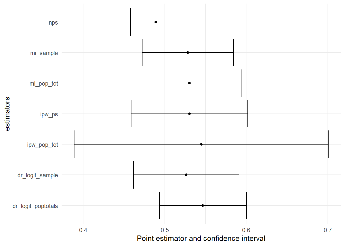

Congratulations! 🎉

You’ve successfully completed these exercises! By now, you should have a solid understanding of how the different approaches work and how to apply various methodologies.

To keep building your skills, here are a few extra exercises:

Explore the outputs: Take some time to analyze the results from the different models, such as the weights, predictions, and more
Try out different specifications: Use a different model than logistic regressioin
Apply what you’ve learned: Try using these models on your own data to see how they perform in real-world scenarios
Take on the Election Challenge: and try to predict election results [Add link to the other file]

Bayesian approaches

Multilevel regression and post-stratification

We use the data from from the 2018 Cooperative Cooperative Congressional Election Study, a US nationwide survey designed by a consortium of 60 research teams and administered by YouGov. The data and the guide with information about the survey and the questionnaire area available here.

This tutorial is adapted from the Book MRP Case Studies that you can find here.

Objectives

Estimate the proportion of individuals who support the cut in the Corporate Income Tax rate. The questionnaire item is the following:

Congress considered many changes in tax law over the past two years. Do you support or oppose each of the following?

CC18_325a Taxes – Cut the Corporate Income Tax rate from 39 percent to 21 percent. (Support/Oppose)

Compare the estimates obtained with the unadjasted nonprobability sample, with the estimates we would obtain if we had a large probability sample and the estimates obtained with MRP

The data

The variables are the following:

state : 50 US states
age : Age in classes, 18-29, 30-39, 40-49, 50-59, 60-69, 70+
male : Gender classified as male (1) or Female (2)
eth : Ethnicity classified as (Non-hispanic) White, Black, Hispanic, Other (which also includes Mixed)
educ : Education classified as No HS, HS, Some college, 4-year college, Post-grad
region : Geographical region classified in Northeast, North Central, South, and West
repvote : Republican vote share in the 2016 presidential election

If you follow the book example, some data pre-processing are needed. Here, for simplicity, we use a ready-to-use version of the data.

Before starting, you need to install and load the following packages:

library(tidyverse)
library(rstan)
library(rstanarm)
library(dplyr)
library(readr)

library(ggplot2)
library(bayesplot)
library(ggalt)
library(reshape2)

You have the following dataset available:

statelevel_predictors_df : for each one of the 50 US States contains the repvote and the region
cces_biased_df : a nonprobability sample of size 5.000 from which we obtain un-adjusted estimates and then MRP estimates
cces_all_df : is the full probability sample of size 59.693 observations that we use only for comparison
poststrat_df_full : is the poststratification table with population counts constructed considering the state, the ethniticy, the gender, the age and the education of individuals. As we defined the levels for these variables, the poststratification table must have \(50 \cdot 6 \cdot 2 \cdot 4 \cdot 5 = 12.000\) rows. This means we actually have more rows in the poststratification table than observed units, which necessarily implies that there are some combinations in the poststratification table that we don’t observe in our nonprobability sample. In this example, we ensured that all cells in the poststratification table were included, even if their weight was zero, but this was done solely for illustrative purposes.

statelevel_predictors_df <- read_csv('statelevel_predictors.csv')
load("cces_all_df.rda")
load("cces_biased_df.rda")
load("poststrat_df_full.rda")

Preliminary analyses

Compare the composition of the nonprobability sample with respect to the population characteristics (in the poststratification table)
Produce plots and tables.

One of the possible solutions follows.

Click here to show the solution

age_sample <-
  cces_biased_df %>% 
  mutate(age = factor(age, ordered = FALSE)) %>% 
  group_by(age) %>% 
  summarise(n = n()) %>% 
  mutate(Sample = n /sum(n))


age_post <- poststrat_df %>% 
  mutate(age = factor(age, ordered = FALSE)) %>% 
  group_by(age) %>% 
  summarise(n_post = sum(n)) %>% 
  mutate(Population = n_post/sum(n_post))

age <-
  inner_join(age_sample, age_post, by = "age") %>% 
  select(age, Sample, Population)


age_plot <- ggplot() + ylab("") + xlab("Proportion") + 
  theme_bw() + coord_flip()  +
  geom_dumbbell(data = age, aes(y = age, x = Sample, xend = Population)) +
  geom_point(
    data = melt(age, id = "age"),
    aes(y = age, x = value, color = variable),
    size = 2
  ) +
  scale_x_continuous(limits = c(0, 0.35), 
                     breaks = c(0, .1, .2, .3)) + 
  theme(legend.position = "none") + 
  ggtitle("Age")

# Gender
male_sample <-
  cces_biased_df %>% 
  group_by(male) %>% 
  summarise(n = n()) %>% 
  mutate(Sample = n / sum(n))

male_post <-
  poststrat_df %>% 
  group_by(male) %>% 
  summarise(n_post = sum(n)) %>% 
  mutate(Population = n_post / sum(n_post))

male <-
  inner_join(male_sample, male_post, by = "male") %>% 
  select(male, Sample, Population) %>%
  mutate(male = factor(
    male,
    levels = c(-0.5,+0.5),
    labels = c("Female", "Male")
  ))


male_plot <- ggplot() + ylab("") + xlab("") + 
  theme_bw() + coord_flip()  +
  geom_dumbbell(data = male, aes(y = male, x = Sample, xend = Population)) +
  geom_point(
    data = melt(male, id = "male"),
    aes(y = male, x = value, color = variable),
    size = 2
  ) +
  scale_x_continuous(limits = c(0, 0.6),
                     breaks = c(0, .2, .4, .6)) + 
  theme(legend.position = "none") + ggtitle("Gender")


# Ethnicity
ethnicity_sample <-
  cces_biased_df %>% 
  group_by(eth) %>% 
  summarise(n = n()) %>% 
  mutate(Sample = n / sum(n))

ethnicity_post <-
  poststrat_df %>% 
  group_by(eth) %>% 
  summarise(n_post = sum(n)) %>%
  mutate(Population = n_post / sum(n_post))

ethnicity <-
  inner_join(ethnicity_sample, ethnicity_post, by = "eth") %>% 
  select(eth, Sample, Population)


ethnicity$eth <- factor(
  ethnicity$eth,
  levels = c("Black", "Hispanic", "Other", "White"),
  labels = c("Black", "Hispanic", "Other", "White")
)


ethnicity_plot <- ggplot() + ylab("") + xlab("") + 
  theme_bw() + coord_flip()  +
  geom_dumbbell(data = ethnicity, aes(y = eth, x = Sample, xend = Population)) +
  geom_point(
    data = melt(ethnicity, id = "eth"),
    aes(y = eth, x = value, color = variable),
    size = 2
  ) +
  scale_x_continuous(limits = c(0, 0.9), 
                     breaks = c(0, .2, .4, .6, 0.8)) + 
  theme(legend.position = "none") + ggtitle("Ethnicity")


# Education
educ_sample <-
  cces_biased_df %>% 
  mutate(educ = factor(educ, ordered = FALSE)) %>% 
  group_by(educ) %>% 
  summarise(n = n()) %>% 
  mutate(Sample = n / sum(n))


educ_post <-
  poststrat_df %>% 
  mutate(educ = factor(educ, ordered = FALSE)) %>% 
  group_by(educ) %>% 
  summarise(n_post = sum(n)) %>% 
  mutate(Population = n_post /sum(n_post))


educ <- inner_join(educ_sample, educ_post, by = "educ") %>% 
  select(educ, Sample, Population)



educ$educ <- factor(
  educ$educ,
  levels = c("No HS", "HS", "Some college", "4-Year College", "Post-grad"),
  labels = c("No HS", "HS", "Some\nCollege", "4-year\nCollege", "Post-grad")
)


educ_plot <- ggplot() + ylab("") + xlab("") + 
  theme_bw() + coord_flip()  +
  geom_dumbbell(data = educ, aes(y = educ, x = Sample, xend = Population)) +
  geom_point(
    data = melt(educ, id = "educ"),
    aes(y = educ, x = value, color = variable),
    size = 2
  ) +
  scale_x_continuous(limits = c(0, 0.33), 
                     breaks = c(0, .1, .2, .3)) + 
  theme(legend.position = "none") + ggtitle("Education")

# State
state_sample<- cces_biased_df %>% 
  group_by(state) %>% 
  summarise(n = n()) %>% 
  mutate(Sample = n/sum(n))


state_post <- poststrat_df %>% 
  group_by(state) %>% 
  summarise(n_post = sum(n)) %>% 
  mutate(Population = n_post/sum(n_post))

state <- full_join(state_sample, state_post, by = "state")

state=state %>% inner_join(statelevel_predictors_df %>% select(state,repvote))

Joining with `by = join_by(state)`

states_order <- state$repvote

state$state <- fct_reorder(state$state, states_order)

ggpubr::ggarrange(age_plot, male_plot, ethnicity_plot, educ_plot, nrow=1,common.legend = TRUE, legend="bottom")

state %>% 
  ggplot() + 
  ylab("") + xlab("Proportion") + theme_bw() + coord_flip()  + 
  geom_dumbbell(aes(y = state, x = Sample, xend = Population)) +
  geom_point(aes(y = state, x = Sample, color = "Sample"), size = 2) +
  geom_point(aes(y = state, x = Population, color = "Population"), size = 2) +
  scale_x_continuous(limits = c(0, 0.13), breaks = c(0, .025, .05, .075, .1, .125)) + ggtitle("State") + 
  theme(legend.position = "bottom", legend.title=element_blank())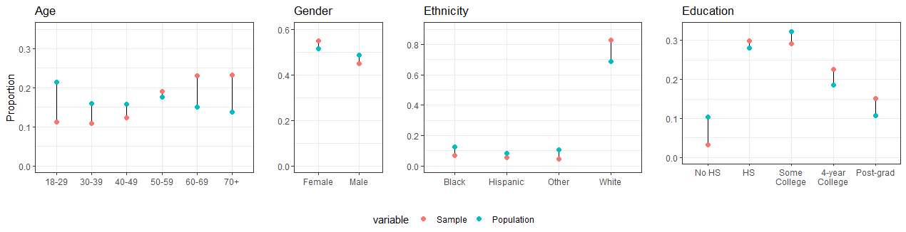

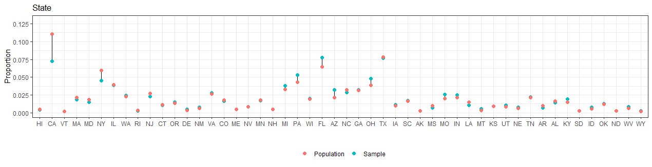
We can see that in the nonprobability samples individuals tends to be older, male, white, less educated and from Republican states.

The Mister: MR

In this section you need to implement a multilevel regression in order to predict the outcome (taxred) based on a set of factors.
Use the stan_gmler function
Include in the model varying intercepts (1 | x) for: age, eth, educ, and state
Include interactions (1 | x1:x2) between male and eth , educ and age and educ and eth
Include as state-level predictors also repvote and region
Use a logistic model

Click here to show the solution

library(rstanarm)
fit <- stan_glmer(taxred ~ (1 | state) + (1 | eth) + (1 | educ) + (1 | age) + male +
                    (1 | male:eth) + (1 | educ:age) + (1 | educ:eth) +
                    repvote + factor(region),
                  family = binomial(link = "logit"),
                  data = cces_biased_df,
                  prior = normal(0, 1, autoscale = TRUE),
                  prior_covariance = decov(scale = 0.50),
                  adapt_delta = 0.99,
                  refresh = 0,
                  seed = 1010)

Running this code might be computational expensive, thus you can directly load the data with the results:

fit <- readRDS("my_fit.rds")

The P: Postststratification

The second step is to poststratify.

Draw 4000 values from the posterior predictive distribution using posterior_epred using the poststrat_df
Compute the vector of MRP estimates for the 4000 draws, remember from the slides pred * n/N . Note that the predictions comes from 4000 draws from the predictive distribution, thus you have a matrix
Compute the final general MRP estimates taking the mean and the sd

Click here to show the solution

epred_mat <- posterior_epred(fit, newdata = poststrat_df, draws = 4000)
mrp_estimates_vector <- epred_mat %*% poststrat_df$n / sum(poststrat_df$n)
mrp_estimate <- c(mean = mean(mrp_estimates_vector), sd = sd(mrp_estimates_vector))

Compute the mean and the standard error from the row nonprobability data and from the larger probability sample data (for a bernoulli distribution it is sqrt(p*(1-p)/n)

Click here to show the solution

get_se_bernoulli <- function(p, n){
  return(sqrt(p*(1-p)/n))
}
cces_estimate <- c(mean = mean(cces_biased_df$taxred), se = get_se_bernoulli(mean(cces_biased_df$taxred), nrow(cces_biased_df)))
full_cces_estimate <- c(mean = mean(cces_all_df$taxred), se = get_se_bernoulli(mean(cces_all_df$taxred), nrow(cces_all_df)))

Compute the MRP and the unadjasted estimates for each of the 50 US states
Compute the estimates for each of the 50 US States using the probability sample data
Use the following code. Take your time to understand it

Click here to show the solution

state_abb <- datasets::state.abb

states_df <- data.frame(
  state = state_abb,
  mrp_estimate = NA,
  mrp_estimate_se = NA,
  cces_estimate = NA,
  cces_estimate_se = NA,
  full_cces_estimate = NA,
  full_cces_estimate_se = NA,
  n_sample = NA,
  n_full = NA
)

for (i in 1:nrow(states_df)) {
  filtering_condition <-
    which(poststrat_df$state == states_df$state[i])
  state_epred_mat <- epred_mat[, filtering_condition]
  k_filtered <- poststrat_df[filtering_condition,]$n
  mrp_estimates_vector <-
    state_epred_mat %*% k_filtered / sum(k_filtered)
  states_df %>% count(state)
  
  # MRP estimate
  states_df$mrp_estimate[i] <- mean(mrp_estimates_vector)
  states_df$mrp_estimate_se[i] <- sd(mrp_estimates_vector)
  
  # Biased sample survey unadjusted estimate
  states_df$cces_estimate[i] <-
    mean(filter(cces_biased_df, state == states_df$state[i])$taxred)
  states_df$n_sample[i] <-
    nrow(filter(cces_biased_df, state == states_df$state[i]))
  states_df$cces_estimate_se[i] <-
    get_se_bernoulli(states_df$cces_estimate[i], states_df$n_sample[i])
  
  # Full PS sample survey unadjusted estimate
  states_df$full_cces_estimate[i] <-
    mean(filter(cces_all_df, state == states_df$state[i])$taxred)
  states_df$n_full[i] <-
    nrow(filter(cces_all_df, state == states_df$state[i]))
  states_df$full_cces_estimate_se[i] <-
    get_se_bernoulli(states_df$full_cces_estimate[i], states_df$n_full[i])
}

Compare the results

Compare the results using ggplot

Click here to show the solution

compare1 <- ggplot(data = states_df) +
  geom_point(aes(x = state, y = cces_estimate), color = "#E37B1C") +
  geom_errorbar(
    aes(
      ymin = cces_estimate - 2 * cces_estimate_se,
      ymax = cces_estimate + 2 * cces_estimate_se,
      x = state
    ),
    alpha = .5,
    width = 0,
    color = "#E37B1C"
  ) +
  geom_point(data = states_df,
             aes(x = state, y = mrp_estimate),
             color = "#7B1CE3") +
  geom_errorbar(
    data = states_df,
    aes(
      ymin = mrp_estimate - 2 * mrp_estimate_se,
      ymax = mrp_estimate + 2 * mrp_estimate_se,
      x = state
    ),
    alpha = .5,
    width = 0,
    color = "#7B1CE3"
  ) +
  geom_point(aes(x = state, y = full_cces_estimate), color = "#1CE37B") +
  geom_errorbar(
    data = states_df,
    aes(
      ymin = full_cces_estimate - 2 * full_cces_estimate_se,
      ymax = full_cces_estimate + 2 * full_cces_estimate_se,
      x = state
    ),
    alpha = .5,
    width = 0,
    color = "#1CE37B"
  ) +
  scale_y_continuous(
    breaks = c(0, .25, .5, .75, 1),
    labels = c("0%", "25%", "50%", "75%", "100%"),
    expand = c(0, 0)
  ) +
  coord_cartesian(ylim = c(0, 1)) +
  theme_bw() +
  labs(x = "States", y = "Support") +
  theme(
    legend.position = "none",
    axis.title = element_text(size = 10),
    axis.text.y = element_text(size = 10),
    axis.text.x = element_text(
      angle = 90,
      size = 8,
      vjust = 0.3
    ),
    legend.title = element_text(size = 10),
    legend.text = element_text(size = 10)
  )

compare2 <- ggplot(data = data.frame()) +
  geom_point(aes(y = cces_estimate[1], x = .25), color = "#E37B1C") +
  geom_errorbar(
    data = data.frame(),
    aes(
      y = cces_estimate[1],
      x = .25,
      ymin = cces_estimate[1] - 2 * cces_estimate[2],
      ymax = cces_estimate[1] + 2 * cces_estimate[2]
    ),
    width = 0,
    color = "#E37B1C"
  ) +
  geom_text(
    aes(x = Inf, y = cces_estimate[1] + 0.06, label = "Unadjusted Sample"),
    hjust = -.05,
    size = 4,
    color = "#E37B1C"
  ) +
  geom_point(aes(y = mrp_estimate[1], x = .75), color = "#7B1CE3") +
  geom_errorbar(
    data = data.frame(),
    aes(
      y = mrp_estimate[1],
      x = .75,
      ymin = mrp_estimate[1] - 2 * mrp_estimate[2],
      ymax = mrp_estimate[1] + 2 * mrp_estimate[2]
    ),
    width = 0,
    color = "#7B1CE3"
  ) +
  geom_text(
    data = data.frame(),
    aes(x = Inf, y = mrp_estimate[1] + 0.02, label = "Sample with MRP"),
    hjust = -.05,
    size = 4,
    color = "#7B1CE3"
  ) +
  scale_y_continuous(
    breaks = c(0, .25, .5, .75, 1),
    labels = c("0%", "25%", "50%", "75%", "100%"),
    limits = c(0, 1),
    expand = c(0, 0)
  ) +
  geom_point(data = data.frame(),
             aes(y = full_cces_estimate[1], x = .5),
             color = "#1CE37B") +
  geom_errorbar(
    data = data.frame(),
    aes(
      y = full_cces_estimate[1],
      x = .5,
      ymin = full_cces_estimate[1] - 2 *
        full_cces_estimate[2],
      ymax = full_cces_estimate[1] + 2 *
        full_cces_estimate[2]
    ),
    width = 0,
    color = "#1CE37B"
  ) +
  geom_text(
    data = data.frame(),
    aes(x = Inf, y = full_cces_estimate - 0.04, label = "Complete Survey"),
    hjust = -.06,
    size = 4,
    color = "#1CE37B"
  ) +
  scale_y_continuous(
    breaks = c(0, .25, .5, .75, 1),
    labels = c("0%", "25%", "50%", "75%", "100%"),
    limits = c(0, 1),
    expand = c(0, 0)
  ) +
  scale_x_continuous(
    limits = c(0, 1),
    expand = c(0, 0),
    breaks = c(.25, .75)
  ) +
  coord_cartesian(clip = 'off') +
  theme_bw() +
  labs(x = "Population", y = "") +
  theme(
    legend.position = "none",
    axis.title.y = element_blank(),
    axis.title.x = element_text(size = 10, margin = margin(
      t = 19,
      r = 0,
      b = ,
      l = 0
    )),
    axis.text = element_blank(),
    axis.ticks = element_blank(),
    legend.title = element_text(size = 10),
    legend.text = element_text(size = 10),
    plot.margin = margin(5.5, 105, 5.5, 5.5, "pt")
  )

Scale for y is already present.
Adding another scale for y, which will replace the existing scale.

bayesplot_grid(compare1,compare2, 
               grid_args = list(nrow=1, widths = c(5,1.4)))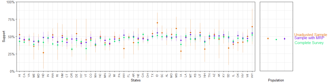

Congratulations! 🎉

You’ve made it through these exercises! By now, you should have a solid understanding of how MRP works—or at least a pretty good idea.

Bayesian inference can be a bit tricky, but don’t worry if it feels like a lot to take in. You’re on the right track!

To improve your Bayesian skills, here are some excellent resources:

Doing Bayesian Data Analysis: by John K. Kruschke
Regression and Other stories: by Andrew Gelman, Jennifer Hill, and Aki Vehtari
UU Summer School: A gentle introduction to Bayesian estimation

Acknowledgments

Some of the exercises are adapted from:

Valliant, R., Dever, J. A., & Kreuter, F. (2018). Practical tools for designing and weighting survey samples (Vol. 1). New York: Springer.
The MRP Case Studies online book that you can find here.