Survey weighting

Introduction

Adjusting for Nonresponse

Propensity score weighting and stratification

Weighting: Creating tailored weights

In this exercise we are going to create tailored weights for a survey dataset. We will use the NHANES dataset, which is a survey dataset from the National Health and Nutrition Examination Survey.

This example is adapted from the course Creating Tailored Weights held by Understanding Society. You can find their implementation in Stata Here. Here we replicate this example in R.

The variables that define the sampling design characteristics are:

• sampl: an ID variable
• stratid: a stratification variable
• location: a clustering variable
• finalwgt: a design weight

The specific task is now, to create a tailored weight for the variable hdresult, which contains serum levels of high-density lipoproteins (HDL). However, only 8708 out of 10,337 entries are valid. We will adjust for this missingness through a tailored weight. We assume that all people are eligible to have a valid value for hdresult and that those who don’t have the value are nonrespondents. To create these tailored weights, we will draw upon the base weight finalwgt and create a weight adjustment.

We will use the following packages

library(haven)
library(tidyverse)
library(survey)

1. Loading the NHANES dataset

• First, load the NHANES dataset into R. The dataset is available through this link in the dta format and can be loaded using the haven package. Then, familiarize yourself with the dataset.

# Load the NHANES II dataset
nhanes2 <- read_dta("https://www.stata-press.com/data/r16/nhanes2f.dta")

2. Create a 0/1 indicator of response

To create a 0/1 indicator of response, where 0 is for nonrespondents and 1 is for respondents, use the hdresult variable. For simplicity treat missing values as non response.

Click here to show the solution

# Create a 0/1 indicator of response
nhanes2 <- nhanes2 %>%
  mutate(resp = ifelse(!is.na(hdresult), 1, 0))
# if hdresult is not missing, set resp to 1, otherwise 0

3. Predict the response using logistic regression

• Select suitable predictors for the logistic regression model. Ensure that the predictors do not have missing values. If they do, impute them with a simple procedure, such as taking their average category or mean.

Click here to show the solution

# Display the summary of the predictors and check if they contain missing values
summary(nhanes2 %>% select(sex, race, age, weight,
                           bpsystol, region, health,
                           heartatk, diabetes, sizplace))

      sex             race            age            weight      
 Min.   :1.000   Min.   :1.000   Min.   :20.00   Min.   : 30.84  
 1st Qu.:1.000   1st Qu.:1.000   1st Qu.:31.00   1st Qu.: 60.67  
 Median :2.000   Median :1.000   Median :49.00   Median : 70.42  
 Mean   :1.525   Mean   :1.144   Mean   :47.56   Mean   : 71.90  
 3rd Qu.:2.000   3rd Qu.:1.000   3rd Qu.:63.00   3rd Qu.: 81.19  
 Max.   :2.000   Max.   :3.000   Max.   :74.00   Max.   :175.88  
                                                                 
    bpsystol         region          health         heartatk      
 Min.   : 65.0   Min.   :1.000   Min.   :1.000   Min.   :0.00000  
 1st Qu.:114.0   1st Qu.:2.000   1st Qu.:3.000   1st Qu.:0.00000  
 Median :128.0   Median :3.000   Median :3.000   Median :0.00000  
 Mean   :130.9   Mean   :2.582   Mean   :3.414   Mean   :0.04577  
 3rd Qu.:142.0   3rd Qu.:4.000   3rd Qu.:4.000   3rd Qu.:0.00000  
 Max.   :300.0   Max.   :4.000   Max.   :5.000   Max.   :1.00000  
                                 NA's   :2       NA's   :2        
    diabetes          sizplace    
 Min.   :0.00000   Min.   :1.000  
 1st Qu.:0.00000   1st Qu.:3.000  
 Median :0.00000   Median :5.000  
 Mean   :0.04828   Mean   :5.166  
 3rd Qu.:0.00000   3rd Qu.:8.000  
 Max.   :1.00000   Max.   :8.000  
 NA's   :2                        

# Checking predictors and imputing missing values
nhanes2 <- nhanes2 %>%
  mutate(
    health = ifelse(is.na(health), 3, health), # impute missing values with 3
    heartatk = ifelse(is.na(heartatk), 0, heartatk), # impute missing values with 0
    diabetes = ifelse(is.na(diabetes), 0, diabetes) # impute missing values with 0
  )

# Display the summary of the predictors again to confirm no missing values
summary(nhanes2 %>% select(sex, race, age, weight, 
                           bpsystol, region, health, 
                           heartatk, diabetes, sizplace))

      sex             race            age            weight      
 Min.   :1.000   Min.   :1.000   Min.   :20.00   Min.   : 30.84  
 1st Qu.:1.000   1st Qu.:1.000   1st Qu.:31.00   1st Qu.: 60.67  
 Median :2.000   Median :1.000   Median :49.00   Median : 70.42  
 Mean   :1.525   Mean   :1.144   Mean   :47.56   Mean   : 71.90  
 3rd Qu.:2.000   3rd Qu.:1.000   3rd Qu.:63.00   3rd Qu.: 81.19  
 Max.   :2.000   Max.   :3.000   Max.   :74.00   Max.   :175.88  
    bpsystol         region          health         heartatk      
 Min.   : 65.0   Min.   :1.000   Min.   :1.000   Min.   :0.00000  
 1st Qu.:114.0   1st Qu.:2.000   1st Qu.:3.000   1st Qu.:0.00000  
 Median :128.0   Median :3.000   Median :3.000   Median :0.00000  
 Mean   :130.9   Mean   :2.582   Mean   :3.414   Mean   :0.04576  
 3rd Qu.:142.0   3rd Qu.:4.000   3rd Qu.:4.000   3rd Qu.:0.00000  
 Max.   :300.0   Max.   :4.000   Max.   :5.000   Max.   :1.00000  
    diabetes          sizplace    
 Min.   :0.00000   Min.   :1.000  
 1st Qu.:0.00000   1st Qu.:3.000  
 Median :0.00000   Median :5.000  
 Mean   :0.04827   Mean   :5.166  
 3rd Qu.:0.00000   3rd Qu.:8.000  
 Max.   :1.00000   Max.   :8.000  

• Using the variables you identified run a logistic regression model

Click here to show the solution

# Logistic regression to predict response
model <- glm(resp ~ factor(sex) + factor(race) +
               age + weight + factor(region) +
               factor(diabetes) + factor(sizplace), # predictors
             data = nhanes2, # dataset
             family = binomial()) # binomial family for logistic regression

# Display the summary of the model
summary(model)

Call:
glm(formula = resp ~ factor(sex) + factor(race) + age + weight + 
    factor(region) + factor(diabetes) + factor(sizplace), family = binomial(), 
    data = nhanes2)

Coefficients:
                   Estimate Std. Error z value Pr(>|z|)    
(Intercept)        3.038391   0.203450  14.934  < 2e-16 ***
factor(sex)2       0.133171   0.059871   2.224 0.026129 *  
factor(race)2      0.233674   0.092552   2.525 0.011577 *  
factor(race)3     -0.382336   0.183499  -2.084 0.037197 *  
age               -0.008039   0.001684  -4.774 1.81e-06 ***
weight            -0.008089   0.001926  -4.201 2.66e-05 ***
factor(region)2   -0.200494   0.094796  -2.115 0.034428 *  
factor(region)3   -0.928439   0.091653 -10.130  < 2e-16 ***
factor(region)4   -0.397968   0.093853  -4.240 2.23e-05 ***
factor(diabetes)1 -0.517688   0.113408  -4.565 5.00e-06 ***
factor(sizplace)2 -0.960051   0.113417  -8.465  < 2e-16 ***
factor(sizplace)3 -0.152250   0.120993  -1.258 0.208268    
factor(sizplace)4  0.266558   0.139023   1.917 0.055192 .  
factor(sizplace)5  0.454941   0.175049   2.599 0.009351 ** 
factor(sizplace)6 -0.385489   0.145213  -2.655 0.007939 ** 
factor(sizplace)7  0.693591   0.155897   4.449 8.63e-06 ***
factor(sizplace)8  0.379206   0.110780   3.423 0.000619 ***
---
Signif. codes:  0 '***' 0.001 '**' 0.01 '*' 0.05 '.' 0.1 ' ' 1

(Dispersion parameter for binomial family taken to be 1)

    Null deviance: 9006.6  on 10336  degrees of freedom
Residual deviance: 8425.9  on 10320  degrees of freedom
AIC: 8459.9

Number of Fisher Scoring iterations: 5

• Predict the response probabilities for the respondents

Click here to show the solution

# Predict response probabilities for respondents
nhanes2 <- nhanes2 %>%
  mutate(prob1 = ifelse(resp == 1, 
                        predict(model, type = "response"), 0))
# predict response probability for respondents, set 0 for nonrespondents

4. Create tailored weights

• Create a weight variable cwgt that is the inverse of the predicted response probability for respondents.

Click here to show the solution

# Adjustment for the wave 1 base weight
nhanes2 <- nhanes2 %>%
  mutate(cwgt = ifelse(prob1 != 0, 1/prob1, 0)) 
# if prob1 is not 0, set cwgt to 1/prob1, otherwise 0

• Create the tailored weight newweight by multiplying the base weight finalwgt with the weight adjustment cwgt. Display the summary of the new weight.

Click here to show the solution

# Create the tailored weight
nhanes2 <- nhanes2 %>%
  mutate(newweight = finalwgt * cwgt) 
# create the tailored weight by multiplying finalwgt with cwgt

# Display summary of the new weight
summary(nhanes2$newweight)

   Min. 1st Qu.  Median    Mean 3rd Qu.    Max. 
      0    4437    9626   11303   15878   94397 

5. Compare the old and new weights

• Create the survey design objects for the old and new weights.

Click here to show the solution

# Old weight survey design
design_old <- svydesign(id = ~location, 
                        strata = ~stratid, 
                        weights = ~finalwgt, 
                        data = nhanes2)

# New weight survey design
design_new <- svydesign(id = ~location, 
                        strata = ~stratid, 
                        weights = ~newweight, 
                        data = nhanes2)

• What are the mean estimates of hdresult using the old and new weights?

Click here to show the solution

# Mean estimate of hdresult using old weight
mean_hdresult_old <- svymean(~hdresult, design = design_old, na.rm = TRUE)

# Mean estimate of hdresult using new weight
mean_hdresult_new <- svymean(~hdresult, design = design_new, na.rm = TRUE)

Propensity score stratification

In this exercise you will analyse data from the data from the 2003 National Health Interview Survey (NHIS) used to monitor health conditions in the US. A smaller version of the original dataset is available the PracTools package. It is named named nhis and it includes demographic variables only.

• ID: Identification variable
• stratum: Sample design stratum
• psu: Primary sampling unit
• svywt: Survey weight
• sex: Gender (1 = male; 2 = female)
• age: Age (continuous)
• age_r: Recoded age (3 = 18-24 years; 4 = 25-44 years; 5 = 45-64 years; 6 = 65-69 years; 7 = 70-74 years; 8 = 75 years and older)
• hisp: Hispanic ethnicity (1 = Hispanic; 2 = Non-Hispanic)
• marital: Marital status (1 = Separated; 2 = Divorced; 3 = Married; 4 = Single/never married; 5 = Widowed; 9 = Unknown marital status)
• parents: Parent(s) of sample person present in the family (1 = Mother, no father; 2 = Father, no mother; 3 = Mother and father; 4 = Neither mother nor father)
• parents_r: Parent(s) of sample person present in the family recode (1 = Yes; 2 = No)
• educ: Education (1 = 8th grade or less; 2 = 9-12th grade, no high school diploma; 3 = High school graduate; 4 = General education development (GED) degree recipient; 5 = Some college, no degree; 6 = Associate’s degree, technical or vocational; 7 = Associate’s degree, academic program; 8 = Bachelor’s degree (BA, BS, AB, BBA); 9 = Master’s, professional, or doctoral degree)
• educ_r: Education recode (1 = High school, general education development degree (GED), or less; 2 = Some college; 3 = Bachelor’s or associate’s degree; 4 = Master’s degree & higher)
• race: Race (1 = White; 2 = Black; 3 = Other)
• resp: Respondent (0 = nonrespondent; 1 = respondent)

1. Load the package using the following code

library(PracTools)
data("nhis")

1. Fit unweighted logistic, probit and c-log-log models to the resp variable

• Use the covariates age, sex, hisp and race

Click here to show the solution

logit=glm (resp ~ age + as.factor(sex) + as.factor(hisp) + as.factor(race),
           family=binomial(link = "logit"),
           data=nhis)

probit=glm (resp ~ age + as.factor(sex) + as.factor(hisp) + as.factor(race),
            family=binomial(link = "probit"),
            data=nhis)

cloglog=glm (resp ~ age + as.factor(sex) + as.factor(hisp) + as.factor(race),
             family=binomial(link = "cloglog"),
             data=nhis)

• Which variables are significant predictors in each of the models?

Look at the regression tables.

Click here to show the solution

We can look at the following table:

	Dependent variable:
	resp
	logistic	probit	glm: binomial
			link = cloglog
	(1)	(2)	(3)
age	-0.010***	-0.006***	-0.006***
	(0.002)	(0.001)	(0.001)
as.factor(sex)2	-0.077	-0.046	-0.044
	(0.070)	(0.042)	(0.041)
as.factor(hisp)2	0.405***	0.246***	0.241***
	(0.088)	(0.054)	(0.054)
as.factor(race)2	-0.212**	-0.128**	-0.124**
	(0.098)	(0.060)	(0.059)
as.factor(race)3	-0.352**	-0.216**	-0.220**
	(0.160)	(0.098)	(0.100)
Constant	1.015***	0.622***	0.272***
	(0.114)	(0.069)	(0.068)
Observations	3,911	3,911	3,911
Log Likelihood	-2,400.759	-2,400.822	-2,400.990
Akaike Inf. Crit.	4,813.519	4,813.644	4,813.980
Note:	p<0.1; p<0.05; p<0.01

All variables (including the intercept) are significant in all models, except for sex.

• Compare the predicted probabilities from the three models. You can make a table or a plot. Predicted probabilities are in $fitted.values

Click here to show the solution

library(kableExtra)
pred.logit=logit$fitted.values
pred.probit=probit$fitted.values
pred.cloglog=cloglog$fitted.values

We can compare each predicted probabilities against the other:

#This is in base R but you can use ggplot2
par(mfrow = c(1, 3))
plot(pred.logit,pred.probit,xlim=c(0.4,0.8),ylim=c(0.4,0.8))
abline(0,1, col="blue",lwd=2)

plot(pred.logit,pred.cloglog,xlim=c(0.4,0.8),ylim=c(0.4,0.8))
abline(0,1, col="blue",lwd=2)

plot(pred.probit,pred.cloglog,xlim=c(0.4,0.8),ylim=c(0.4,0.8))
abline(0,1, col="blue",lwd=2)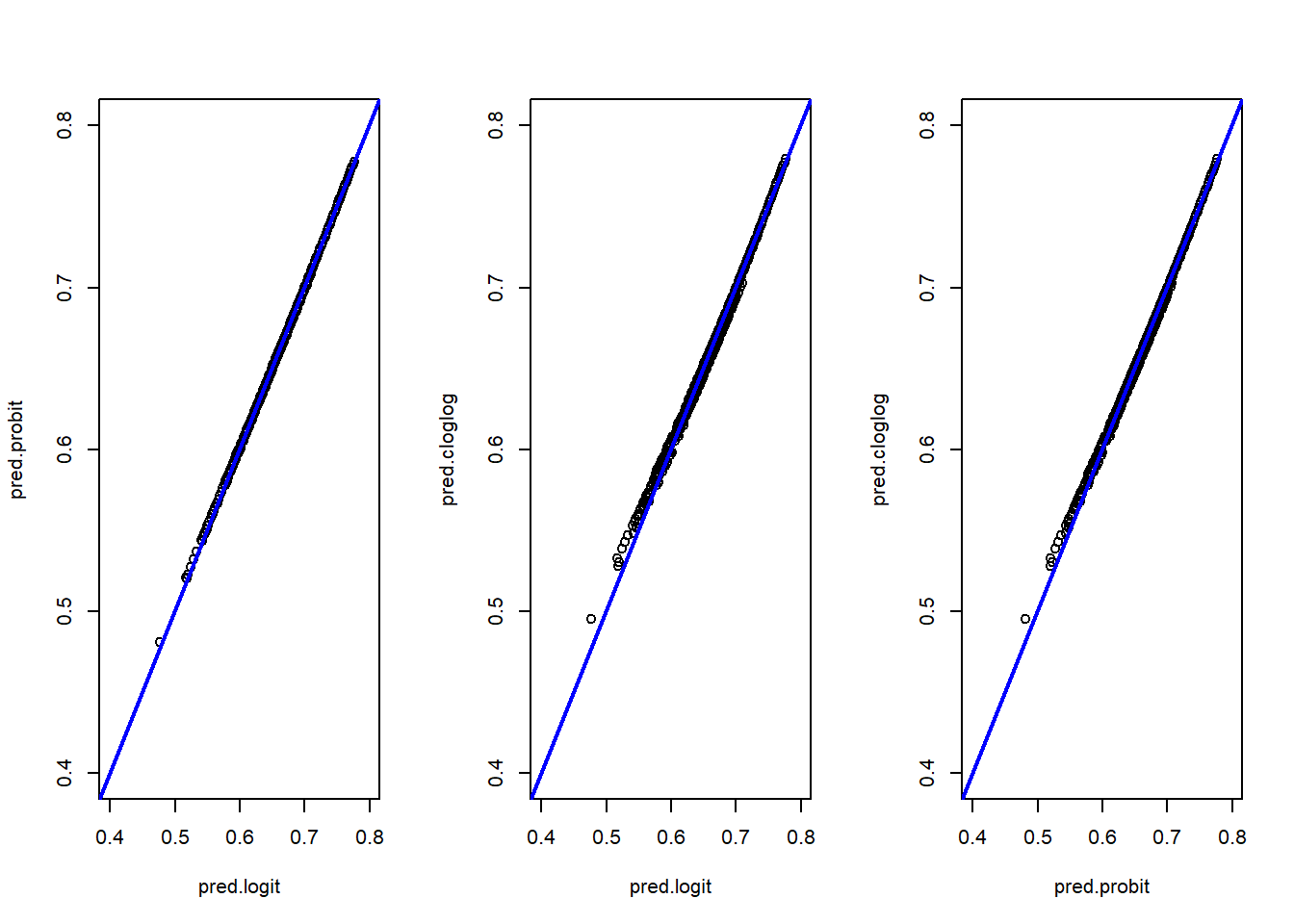

We can make a summary table:

summary(pred.logit) %>% 
  bind_rows(summary(pred.probit)) %>% 
  bind_rows(summary(pred.cloglog)) %>% 
  add_column(model=c("logit","probit","cloglog"),.before=1) %>%
  kable() %>% 
  kable_styling(latex_options = "HOLD_position")

model	Min.	1st Qu.	Median	Mean	3rd Qu.	Max.
logit	0.4769137	0.6585878	0.6924415	0.6901048	0.7260404	0.7765047
probit	0.4808753	0.6584612	0.6919716	0.6900877	0.7258562	0.7773489
cloglog	0.4951173	0.6585117	0.6917511	0.6900942	0.7255815	0.7791557

And some boxplots:

boxplot(pred.logit,pred.probit,pred.cloglog,
        main="Boxplot of predicted probabilities",
        xlab="Model",
        ylab="Pred. Prob.",
        col="dodgerblue",
        border="black")
axis(1,at=c(1,2,3),labels=c("logit","probit","cloglog"))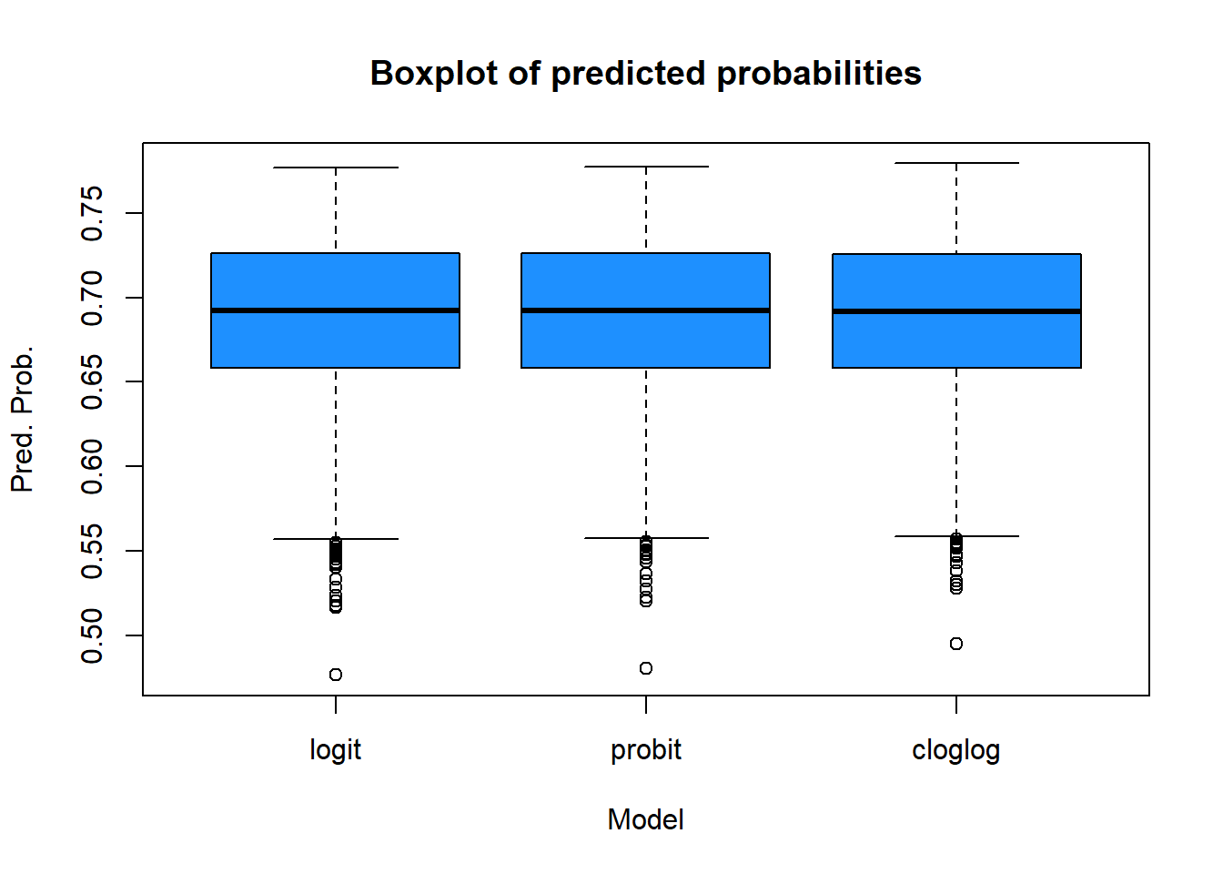

The three models produce very similar results. The logit and probit models are almost identical, while the cloglog model shows slight differences, particularly at the extreme low end of the predicted probabilities (as seen in the scatter plots and box plots). Analyzing the min-max values and quartiles leads to the same conclusion: the models are closely aligned overall.

3. Use the predicted response probabilities from the logistic regression that used all covariates and create two versions of propensity classes:

• Five classes with an equal number of respondents plus nonrespondents in each. Use pclass in order to make classes.

Click here to show the solution

p.class5 <- pclass(formula=resp ~ age + as.factor(sex) + as.factor(hisp) + as.factor(race),
                   type="unwtd",data=nhis,link="logit", numcl=5)

• Ten classes. Report the breaks used for the five and ten classes and the number of cases assigned to each class. (Check to see that all cases were assigned a non-missing class value. Use the parameter `useNA=“always”` in table in order to see whether NAs were created.)

Click here to show the solution

p.class10 <- pclass(formula=resp ~ age + as.factor(sex) + as.factor(hisp) + as.factor(race),
                    type="unwtd",data=nhis,link="logit", numcl=10)

4. How do the five and ten classes compare to each other?

Click here to show the solution

table(p.class5$p.class,useNA="always") %>% 
  kable(col.names = c("Boundaries","Count of persons")) %>% 
  kable_styling(latex_options = "HOLD_position")

Boundaries	Count of persons
[0.477,0.651]	783
(0.651,0.68]	782
(0.68,0.706]	782
(0.706,0.734]	782
(0.734,0.777]	782
NA	0

table(p.class10$p.class,useNA="always") %>% 
  kable(col.names = c("Boundaries","Count of persons")) %>% 
  kable_styling(latex_options = "HOLD_position")

Boundaries	Count of persons
[0.477,0.629]	392
(0.629,0.651]	391
(0.651,0.665]	391
(0.665,0.68]	391
(0.68,0.692]	391
(0.692,0.706]	391
(0.706,0.72]	391
(0.72,0.734]	391
(0.734,0.75]	391
(0.75,0.777]	391
NA	0

All cases have been assigned a non-missing class value, and the number of individuals is nearly as expected. The 10 classes also show greater homogeneity.

5. How do the class adjustments compare to using the inverses of individual propensity estimates as adjustments?

Click here to show the solution

data5=data.frame(p.class5)

ggplot(data5, aes(x=p.class, y=propensities)) +
  geom_boxplot(alpha=0.7) +
  stat_summary(fun.y=mean, geom="point", shape=20, size=4, color="red", fill="red") +
  theme(legend.position="none") +
  scale_fill_brewer(palette="Set1")+theme_bw()

Warning: The `fun.y` argument of `stat_summary()` is deprecated as of ggplot2 3.3.0.
ℹ Please use the `fun` argument instead.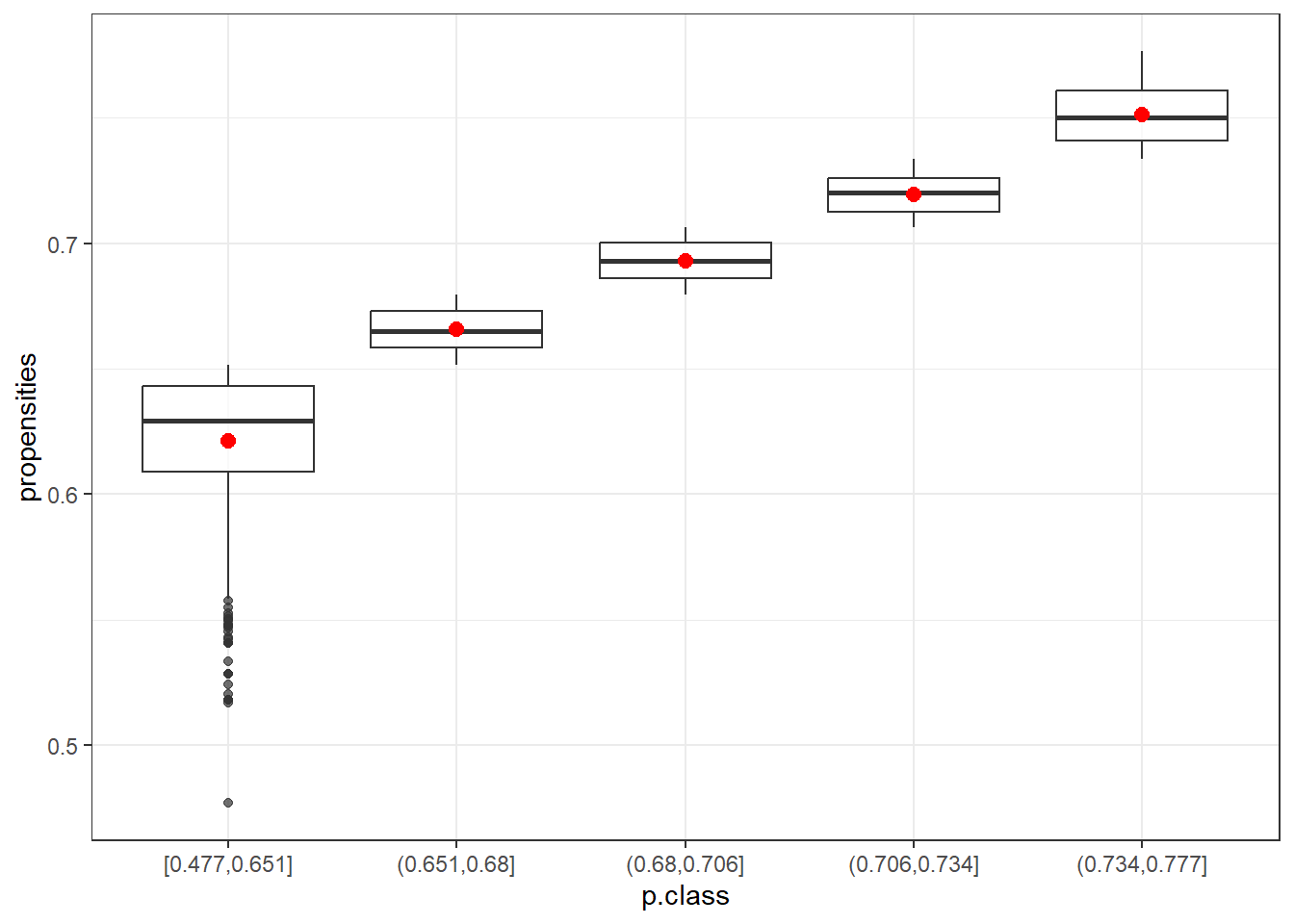

data10=data.frame(p.class10)

ggplot(data10, aes(x=p.class, y=propensities)) +
  geom_boxplot(alpha=0.7) +
  stat_summary(fun.y=mean, geom="point", shape=20, size=4, color="red", fill="red") +
  theme(legend.position="none") +
  scale_fill_brewer(palette="Set1")+theme_bw()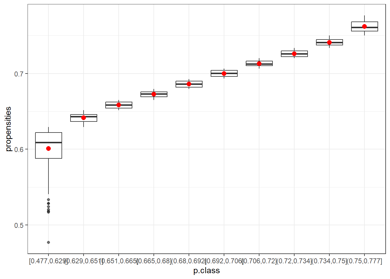

The box plots show that the first class (in both cases) is the most variable. After that, the range of propensities decreases. Using the mean (red) or the median helps to smooth out more extreme adjustments, which is especially beneficial for the first class. This highlights the advantage of using classes instead of raw propensity values.

6. Which set of adjustment values would you recommend and why?

Think about it and discuss it in groups.

Extra exercises

If the ranges of estimated propensities in each class is small, you can use a single propensity value for each class. There are several options:

Calculate the five alternative values of NR weight adjustment shown in the box below.

For the weighted adjustments, use the svywt variable. Discuss how the five alternative values of adjustments compare within the two models with five and ten classes compare to each other

Five ways of estimating the class response propensity

1. Unweighted average: \(\hat{\phi}_c = \frac{1}{n_c} \sum_{i \in s_c} \hat{\phi}(x_i)\) where \(n_c\) is the unweighted number of cases in class c

2. Weighted average: \(\hat{\phi}_c = \frac{\sum_{i \in s_c}d_i\hat{\phi}(x_i)}{\sum_{i \in s_c}d_i}\) where \(d_i\) is the base weight and the sum of \(d_i\) is the estimated number of population units in class \(c\)

3. Unweighted response rate: \(\hat{\phi}_c = n_{cR}/n_c\) where \(n_{cR}\) is the unweighted number of respondents in class c

4. Weighted response rate: \(\sum_{i \in s_{cR}}d_i/\sum_{i \in s_c}d_i\) where \(n_c\) is the unweighted number of cases in class c

5. Unweighted median: \(\hat{\phi}_c = median [\hat{\phi}(x_i)]_{i \in s_c}\) where \(n_c\) is the unweighted number of cases in class c

Click here to show the solution

We compute the results for the case with 5 an 10 class respectively.

unw5=by(data=p.class5$propensities, p.class5$p.class, mean)

weigh5=by(data=data.frame(preds=p.class5$propensities, wt=nhis[,"svywt"]),
          p.class5$p.class, function(x) {weighted.mean(x$preds,x$wt)})

unw.resp5=by(as.numeric(nhis[,"resp"]), p.class5$p.class, mean)

weigh.resp5=by(data=data.frame(resp=as.numeric(nhis[,"resp"]),wt=nhis[,"svywt"]),
               p.class5$p.class, function(x) {weighted.mean(x$resp,x$wt)})

med5=by(p.class5$propensities, p.class5$p.class, median)

unw10=by(data=p.class10$propensities, p.class10$p.class, mean)

weigh10=by(data=data.frame(preds=p.class10$propensities, wt=nhis[,"svywt"]),
           p.class10$p.class, function(x) {weighted.mean(x$preds,x$wt)})

unw.resp10=by(as.numeric(nhis[,"resp"]), p.class10$p.class, mean)

weigh.resp10=by(data=data.frame(resp=as.numeric(nhis[,"resp"]),wt=nhis[,"svywt"]),
                p.class10$p.class, function(x) {weighted.mean(x$resp,x$wt)})

med10=by(p.class10$propensities, p.class10$p.class, median)

Then, we compare the results considering the following tables:

	Count of persons	Unw. avg. prop.	W. avg. prop.	Unw. RR	W. RR	Median
[0.477,0.651]	783	0.6211	0.6237	0.6271	0.6463	0.6294
(0.651,0.68]	782	0.6656	0.6656	0.6662	0.6677	0.6651
(0.68,0.706]	782	0.6930	0.6933	0.6739	0.6859	0.6929
(0.706,0.734]	782	0.7195	0.7196	0.7353	0.7338	0.7201
(0.734,0.777]	782	0.7514	0.7521	0.7481	0.7623	0.7503

	Count of persons	Unw. avg. prop.	W. avg. prop.	Unw. RR	W. RR	Median
[0.477,0.629]	392	0.6008	0.6026	0.5765	0.5915	0.6090
(0.629,0.651]	391	0.6415	0.6416	0.6777	0.6930	0.6430
(0.651,0.665]	391	0.6586	0.6585	0.6547	0.6577	0.6586
(0.665,0.68]	391	0.6727	0.6727	0.6803	0.6820	0.6731
(0.68,0.692]	391	0.6861	0.6862	0.6803	0.6833	0.6860
(0.692,0.706]	391	0.6999	0.7000	0.6650	0.6857	0.7002
(0.706,0.72]	391	0.7131	0.7131	0.7161	0.7092	0.7126
(0.72,0.734]	391	0.7259	0.7260	0.7545	0.7562	0.7260
(0.734,0.75]	391	0.7408	0.7407	0.7596	0.7710	0.7411
(0.75,0.777]	391	0.7619	0.7622	0.7366	0.7551	0.7610

Overall, for both 5 and 10 classes, we observe that values generally increase across classes, with all five methods producing similar results. The first and last classes show a wider range of values.

When comparing the results between 5 and 10 classes, the range is narrower in the 10-class scenario. While using more classes can help reduce bias due to nonresponse, it may also lead to higher variances. Typically, 5 classes are recommended when the sample size is not large. In this case, opting for 5 classes seems appropriate.

2. Check covariate balance according to D’Agostino method. Is balancing achieved? Discuss it.

Checking Balance on Covariates - D’Agostino 1998

The idea is simple: after classes are formed, you check if there is a difference in the covariate means. The covariate means should be different between classes but within a class the means of the covariates should be the same for respondents and nonrespondents. This is consistent with the idea that the response propensity is the same for all units withing a class.

To check balance on covariates you need to:

• for quantitative x’s: fit an ANOVA model, where x = p.class + resp + p.class*resp

• for dichtonomous x’s: fit a logistic model, where logit(x) = p.class + resp + p.class*resp

The coefficients on resp and the interaction p.class*respshoud be nonsignificant.

The coefficients on p.classshould be nonzero and different from each other

In addition you can also look at the covariate means table using p.class*resp

Click here to show the solution

This is an example, you can proceed with all the covariates

p.class <- p.class5$p.class


#standard check
chk1 <- glm(age ~ p.class + resp + p.class*resp, data = nhis)

# An additional step is to fit a second model that only inlcudes p.class 
# and test wether chk1 and chk2 are equivalent
chk2 <- glm(age ~ p.class, data = nhis)

summary(chk1)

Call:
glm(formula = age ~ p.class + resp + p.class * resp, data = nhis)

Coefficients:
                          Estimate Std. Error t value Pr(>|t|)    
(Intercept)                60.5000     0.8266  73.189  < 2e-16 ***
p.class(0.651,0.68]        -8.5230     1.2032  -7.083 1.66e-12 ***
p.class(0.68,0.706]       -15.9314     1.2107 -13.159  < 2e-16 ***
p.class(0.706,0.734]      -19.7995     1.2834 -15.427  < 2e-16 ***
p.class(0.734,0.777]      -32.4594     1.3024 -24.923  < 2e-16 ***
resp                       -1.6242     1.0439  -1.556   0.1198    
p.class(0.651,0.68]:resp   -1.1512     1.4957  -0.770   0.4415    
p.class(0.68,0.706]:resp    3.6021     1.5003   2.401   0.0164 *  
p.class(0.706,0.734]:resp   2.5098     1.5494   1.620   0.1053    
p.class(0.734,0.777]:resp   2.3272     1.5632   1.489   0.1366    
---
Signif. codes:  0 '***' 0.001 '**' 0.01 '*' 0.05 '.' 0.1 ' ' 1

(Dispersion parameter for gaussian family taken to be 199.5277)

    Null deviance: 1188013  on 3910  degrees of freedom
Residual deviance:  778357  on 3901  degrees of freedom
AIC: 31823

Number of Fisher Scoring iterations: 2

summary(chk2)

Call:
glm(formula = age ~ p.class, data = nhis)

Coefficients:
                     Estimate Std. Error t value Pr(>|t|)    
(Intercept)           59.4815     0.5053  117.70   <2e-16 ***
p.class(0.651,0.68]   -9.3536     0.7149  -13.08   <2e-16 ***
p.class(0.68,0.706]  -13.5799     0.7149  -19.00   <2e-16 ***
p.class(0.706,0.734] -18.1298     0.7149  -25.36   <2e-16 ***
p.class(0.734,0.777] -30.9150     0.7149  -43.24   <2e-16 ***
---
Signif. codes:  0 '***' 0.001 '**' 0.01 '*' 0.05 '.' 0.1 ' ' 1

(Dispersion parameter for gaussian family taken to be 199.9602)

    Null deviance: 1188013  on 3910  degrees of freedom
Residual deviance:  781044  on 3906  degrees of freedom
AIC: 31827

Number of Fisher Scoring iterations: 2

anova(chk2, chk1, test="Chisq")

Analysis of Deviance Table

Model 1: age ~ p.class
Model 2: age ~ p.class + resp + p.class * resp
  Resid. Df Resid. Dev Df Deviance Pr(>Chi)  
1      3906     781044                       
2      3901     778357  5     2687  0.01937 *
---
Signif. codes:  0 '***' 0.001 '**' 0.01 '*' 0.05 '.' 0.1 ' ' 1

#p-val non significant: balance is fine


#For hispanic you need to recode the data.
new.hisp <- abs(nhis$hisp-2)

#standard check
chk1 <- glm(new.hisp ~ p.class + resp + p.class*resp, family=binomial(link = "logit"), data = nhis)

A numerical note

When running a model to check balance on covariates, you might encounter anomalous results, such as extremely large estimates of standard errors. This could indicate “quasi-complete” separation in the dataset, where one or more observations have a predicted probability very close to 1. In such cases, a parameter estimate may diverge to infinity.

While this poses a significant problem if your goal is to identify covariates associated with the occurrence of a particular characteristic, it does not affect the formation of propensity classes when checking covariate balance.

Congratulations! 🎉

You’ve successfully completed these exercises! By now, you should have a solid understanding of nonresponse.

To keep building your skills, here are a few extra exercises:

• Tailored weights in longitudinal surveys: you can find a Stata tutorial by the UK Understanding Society survey

• Check covariate balance: Do the extra exercise in the propensity score stratification section

• Apply what you’ve learned: Try using these models on your own data

Adjusting for Nonresponse and Coverage

In this exercise we use a larger version of the NHIS dataset that we used in the previous exercise. This dataset, named nhis.large, also contain some health-related variables. We want to estimate the number of persons covered by Medicaid, a type of US governamental assistance for medical care provided to the poor.

We treat the large sample as reference population data. To the purpose of our exercise we also consider a probability sample which is extracted from the NHIS dataset but introducing coverage errors.

Your objective is to perform different adjustment methods, namely, poststratification, raking and GREG calibration.

1. Load the data

Load the nhis.large dataset and recode hisp into three categories (collapse category 4 and 3).

data("nhis.large")
nhis.large1 <- nhis.large %>% 
  mutate(hisp.r = ifelse(hisp==4,3,hisp))
    
load("samdat.rda")

2. Define the sampling design of the sample

   This time specify the weights (N/n) and the finite population correction equal to the sampling fraction (n/N)

Click here to show the solution

N <- nrow(nhis.large1)
n <-nrow(samdat)
d <- rep(N/n, n)
f1 <- rep(n/N, n)

nhis.dsgn <- svydesign(ids = ~0,    # no clusters 
          strata = NULL,    # no strata
          fpc = ~f1,
          data = data.frame(samdat), 
          weights = ~d)

Poststratification

1. Compute the population total in the poststrata defined by age.grp and hisp.r

Click here to show the solution

    N.PS <- xtabs(~ age.grp + hisp.r, data = nhis.large1)

2. Implement postStratify specifying age.grp + hisp.r in the strata argument.

Click here to show the solution

    ps.dsgn <- postStratify(design = nhis.dsgn,
                                strata = ~age.grp + hisp.r,
                                population = N.PS)

Raking

1. Compute the population total for the variable age.grp and hisp.r

   Give appropriate names that match variable names in the raking and GREG models.

Click here to show the solution

N.age <- table(nhis.large1[, "age.grp"])
N.hisp <- table(nhis.large1[, "hisp.r"])

pop.totals <- c('(Intercept)' = N, N.age[-1], N.hisp[-1])

names(pop.totals)=c("(Intercept)","as.factor(age.grp)2",
                    "as.factor(age.grp)3", "as.factor(age.grp)4",
                    "as.factor(age.grp)5" ,"as.factor(hisp.r)2", 
                    "as.factor(hisp.r)3")

2. Implement raking specifying ~ as.factor(age.grp) + as.factor(hisp.r) in the formula argument.

Click here to show the solution

rake.dsgn <- calibrate(design = nhis.dsgn,
                        formula = ~ as.factor(age.grp) + as.factor(hisp.r),
                        calfun = "raking",
                        population = pop.totals)

3. Verify that weights are calibrated for x’s

   Compare the total for age.grp and hisp.r computed using rake.dsgn with the population totals pop.totals

Click here to show the solution

svytotal(~as.factor(age.grp), rake.dsgn, na.rm=TRUE)

                    total SE
as.factor(age.grp)1  5991  0
as.factor(age.grp)2  2014  0
as.factor(age.grp)3  6124  0
as.factor(age.grp)4  5011  0
as.factor(age.grp)5  2448  0

svytotal(~as.factor(hisp.r), rake.dsgn, na.rm=TRUE)

                   total SE
as.factor(hisp.r)1  5031  0
as.factor(hisp.r)2 12637  0
as.factor(hisp.r)3  3920  0

pop.totals

        (Intercept) as.factor(age.grp)2 as.factor(age.grp)3 as.factor(age.grp)4 
              21588                2014                6124                5011 
as.factor(age.grp)5  as.factor(hisp.r)2  as.factor(hisp.r)3 
               2448               12637                3920 

GREG

1. Implement GREG calibration specifying ~ as.factor(age.grp) + as.factor(hisp.r) in the formula argument.

Click here to show the solution

greg.dsgn <- calibrate(design = nhis.dsgn,
                        formula = ~ as.factor(age.grp) + as.factor(hisp.r),
                        calfun = "linear",
                        population = pop.totals)

2. Verify that weights are calibrated for x’s

   Compare the total for age.grp and hisp.r computed using greg.dsgn with the population totals pop.totals

Click here to show the solution

svytotal(~as.factor(age.grp), greg.dsgn, na.rm=TRUE)

                    total SE
as.factor(age.grp)1  5991  0
as.factor(age.grp)2  2014  0
as.factor(age.grp)3  6124  0
as.factor(age.grp)4  5011  0
as.factor(age.grp)5  2448  0

svytotal(~as.factor(hisp.r), greg.dsgn, na.rm=TRUE)

                   total SE
as.factor(hisp.r)1  5031  0
as.factor(hisp.r)2 12637  0
as.factor(hisp.r)3  3920  0

pop.totals

        (Intercept) as.factor(age.grp)2 as.factor(age.grp)3 as.factor(age.grp)4 
              21588                2014                6124                5011 
as.factor(age.grp)5  as.factor(hisp.r)2  as.factor(hisp.r)3 
               2448               12637                3920 

Compare the three methods

Compute the total and the proportion of individuals covered by Medicaid (1=yes, 2=no) using:

1. the original sampling weights

2. the poststratification weights

3. the raking weights

4. the GREG weights

Click here to show the solution

svytotal(~as.factor(medicaid), nhis.dsgn, na.rm=TRUE)

                       total     SE
as.factor(medicaid)1  1823.8 250.18
as.factor(medicaid)2 17190.2 272.46

svytotal(~as.factor(medicaid), ps.dsgn, na.rm=TRUE)

                       total     SE
as.factor(medicaid)1  2492.1 317.07
as.factor(medicaid)2 18638.1 334.06

svytotal(~as.factor(medicaid), rake.dsgn, na.rm=TRUE)

                       total     SE
as.factor(medicaid)1  2555.9 330.66
as.factor(medicaid)2 18516.9 351.43

svytotal(~as.factor(medicaid), greg.dsgn, na.rm=TRUE)

                       total     SE
as.factor(medicaid)1  2534.3 327.89
as.factor(medicaid)2 18539.7 349.04

svyciprop(~as.factor(medicaid)==1, nhis.dsgn, na.rm=TRUE)

                                  2.5%  97.5%
as.factor(medicaid) == 1 0.0959 0.0730 0.1250

svyciprop(~as.factor(medicaid)==1, ps.dsgn, na.rm=TRUE)

                                  2.5%  97.5%
as.factor(medicaid) == 1 0.1179 0.0916 0.1506

svyciprop(~as.factor(medicaid)==1, rake.dsgn, na.rm=TRUE)

                                  2.5%  97.5%
as.factor(medicaid) == 1 0.1213 0.0938 0.1555

svyciprop(~as.factor(medicaid)==1, greg.dsgn, na.rm=TRUE)

                                2.5% 97.5%
as.factor(medicaid) == 1 0.120 0.093 0.154

#true
prop.table(table(nhis.large1[, "medicaid"]))

        1         2 
0.1071194 0.8928806 

The results are quite similar.

Extra exercises

Poststratify vs GREG

Note that applying poststratification with a single variable is equivalent to apply GREG.

1. Apply poststratification and then GREG considering only age.grp.

   Remember to define population total (and names) again.

Click here to show the solution

N.PS1 <- xtabs(~ age.grp, data = nhis.large1)
N <- nrow(nhis.large1)
N.age <- table(nhis.large1[, "age.grp"])


pop.totals1 <- c('(Intercept)' = N, N.age[-1])
names(pop.totals1)=c("(Intercept)","as.factor(age.grp)2",
                    "as.factor(age.grp)3",
                    "as.factor(age.grp)4",
                    "as.factor(age.grp)5")

ps.dsgn1 <- postStratify(design = nhis.dsgn,
                            strata = ~age.grp,
                            population = N.PS1)

greg.dsgn1 <- calibrate(design = nhis.dsgn,
                        formula = ~ as.factor(age.grp),
                        calfun = "linear",
                        population = pop.totals1)

svytotal(~as.factor(medicaid), ps.dsgn1, na.rm=TRUE)

                       total     SE
as.factor(medicaid)1  2211.4 292.27
as.factor(medicaid)2 18919.9 315.91

svytotal(~as.factor(medicaid), greg.dsgn1, na.rm=TRUE)

                       total     SE
as.factor(medicaid)1  2211.4 292.27
as.factor(medicaid)2 18919.9 315.91

2. Continue the GREG exercise and trim your weights to be between 30 and 65

Click here to show the solution

greg.trim <- trimWeights(design = greg.dsgn,
lower = 30,
upper = 65,
strict = TRUE)

svytotal(~as.factor(medicaid), greg.dsgn, na.rm=TRUE)

                       total     SE
as.factor(medicaid)1  2534.3 327.89
as.factor(medicaid)2 18539.7 349.04

svytotal(~as.factor(medicaid), greg.trim, na.rm=TRUE)

                       total     SE
as.factor(medicaid)1  2502.3 323.26
as.factor(medicaid)2 18569.2 345.89

3. Repeat the GREG calibration specifying that the final weights should be between 0.5 and 1.5 times the original weights. Does the calibration work or fail?

Hint: Use bounds = c(0.5,1.5)

Click here to show the solution

greg.bound <- calibrate(design = nhis.dsgn,
                        formula = ~ as.factor(age.grp) + as.factor(hisp.r),
                        calfun = "linear",
                        population = pop.totals,
                        bounds = c(0.5,1.5))

The calibration algorithm fails.

Congratulations! 🎉

You’ve successfully completed these exercises! By now, you should have a solid understanding of survey weighting.

To keep building your skills, here are a few extra suggesions:

• Have a look at the extra exercises: try out different bounds

• Apply what you’ve learned: Try using these models on your own data

• The Election Challange: Apply these methods in Day 4, to correct for selection bias

Acknowledgments

Some of the exercises are adapted from:

• Valliant, R., Dever, J. A., & Kreuter, F. (2018). Practical tools for designing and weighting survey samples (Vol. 1). New York: Springer.

• Creating Tailored Weights - by Understanding Society